Simulate within-host evolution with wavess

wavess is an individual-based discrete-time within-host evolution simulator. We assume that all virus life cycles within the infection are synchronized into generations. Each generation is one full virus life cycle, from infecting a cell to exiting the cell.

In this vignette, we focus on how to simulate within-host evolution using the run_wavess() function. We will be using the HIV ENV gp120 gene as an example. Please note that the default arguments were set with this particular organism and genomic region in mind. If you’d like to simulate something else, you may have to modify certain parameters. However, if you are interested in this gene in particular, you can probably use most of the defaults including the founder and reference sequences provided as examples.

A note about using the simulation output

Before we get started, I just want to note that the output of these simulations is stochastic, meaning they will be different each time it is run. You can set a seed for reproducibility and troubleshooting if you’d like, but for the vast majority of applications, you will want to run many replicates of a given simulation scenario with different seeds (random is okay) to get a reasonable sense of what dynamics are observed. You will also want to check the simulation outputs to see if they are giving you reasonable/expected results that conform to your prior knowledge about the system you’re simulating. If the output does not seem right, you might have to tweak the input parameters to work for your particular system. We go into more detail about analyzing the model output in a separate vignette (see vignette("analyze_output")).

Load libraries

First, we have to load the wavess library and a few additional libraries that we’ll use for this vignette:

library(wavess)
library(ape)
library(dplyr)
#> 
#> Attaching package: 'dplyr'
#> The following object is masked from 'package:ape':
#> 
#>     where
#> The following objects are masked from 'package:stats':
#> 
#>     filter, lag
#> The following objects are masked from 'package:base':
#> 
#>     intersect, setdiff, setequal, union
library(ggplot2)

Create Python virtual environment

Next, we must create a Python virtual environment. The virtual environment is required because the underlying code of run_wavess() is written in Python. You only have to create the virtual environment once on each machine.

create_python_venv()
#> Warning in create_python_venv(): Skipped installation of the following
#> packages: numpyscipypandas Use `force` to force installation or update.

Prepare input data

Next, we must generate the input data. If you’re interested in learning more about how to prepare the input data, please see the corresponding vignette (see vignette("prepare_input_data")).

We will only simulate 300 generations with sampling every 100 generations so the simulation doesn’t take too long to run.

pop <- define_growth_curve(n_gens = 300)
samp <- define_sampling_scheme(sampling_frequency_active = 100, sampling_frequency_latent = 100) |> filter(day <= 300)
founder_ref <- extract_seqs(hxb2_cons_founder,
  founder = "B.US.2011.DEMB11US006.KC473833",
  ref = "CON_B(1295)",
  start = 6225, end = 7787
)
gp120 <- slice_aln(hxb2_cons_founder, 6225, 7787)
epi_probs <- get_epitope_frequencies(env_features$Position)
ref_founder_map <- map_ref_founder(gp120,
  ref = "B.FR.83.HXB2_LAI_IIIB_BRU.K03455",
  founder = "B.US.2011.DEMB11US006.KC473833"
)
epitope_locations <- sample_epitopes(epi_probs,
  ref_founder_map = ref_founder_map
)
#> 16 resamples required

Simplest way to `run_wavess()`

The simplest way to simulate within-host evolution is to use all of the defaults, and only input the population growth and sampling scheme, founder sequence, and nucleotide substitution probabilities.

Please note that the total population size simulated greatly influences the simulation output.

required_args_only <- run_wavess(
  inf_pop_size = pop,
  samp_scheme = samp,
  founder_seqs = rep(founder_ref$founder, 10)
)

Here, we simulate one founder sequence. You may simulate more, but you will have to ensure that they are the same length, do not include gaps, and are codon-aligned. You will also have to modify the input growth curve to start with the correct number of cells. See vignette('prepare_input_data') for more details.

The output format of run_wavess() is a list of length four containing a tibble of various counts, the fitness of the sampled viruses, and the DNA sequences of the sampled viruses from the active and latent reservoir:

names(required_args_only)
#> [1] "counts"      "fitness"     "seqs_active" "seqs_latent"

Note that, if no latent cells are sampled, then the length of the list will be three instead, with no sequences from latent cells.

The counts tibble contains the following columns:

generation: generation that number of events was recorded and sequences were sampled
active_cell_count: active cell count
latent_cell_count: latent cell count
active_turned_latent: number of active cells that became latent
latent_turned_active: number of latent cells that became active
latent_died: number of latent cells that died
latent_proliferated: number of latent cells that proliferated
number_mutations: number of mutations across all sequences
number_recombinations: number of infected cells with at least one recombination event
mean_fitness_active: mean fitness of active cells
mean_conserved_active: mean conserved sites fitness of active cells
mean_b_immune_active: mean antibody immune fitness of active cells
mean_t_immune_active: mean cytotoxic T-lymphocyte (CTL) immune fitness of active cells
mean_replicative_active: mean replicative fitness (comparison to ref_seq) of active cells

required_args_only$counts
#> # A tibble: 4 × 15
#>   generation active_cell_count latent_cell_count active_turned_latent
#>        <int>             <int>             <int>                <int>
#> 1          0                10                 0                    0
#> 2        100              2000               102                    1
#> 3        200              2000               161                    1
#> 4        300              2000               193                    2
#> # ℹ 11 more variables: latent_turned_active <int>, latent_died <int>,
#> #   latent_proliferated <int>, number_mutations <int>,
#> #   number_recombinations <int>, mean_fitness_active <dbl>,
#> #   mean_conserved_active <dbl>, mean_b_immune_active <dbl>,
#> #   mean_t_immune_active <dbl>, mean_replicative_active <dbl>,
#> #   mean_immune_active <dbl>

As you can see, the default values for run_wavess() include latency, mutations, and dual infections (which lead to recombination), but no fitness costs.

The fitness tibble contains a row for each sampled sequence (all from the active pool) and the following columns:

generation: generation that the virus was sampled in
seq_id: sequence id (corresponds to the sequence name below). Note that the same value for different generations does not say anything about the ancestral relationship between the viruses.
immune: virus immune fitness
conserved: virus conserved fitness
replicative: virus replicative fitness (compared to a reference)
overall: overall fitness (the other three multiplied together)

required_args_only$fitness
#> # A tibble: 80 × 8
#>    generation seq_id   b_immune t_immune conserved replicative overall immune
#>    <chr>      <chr>       <dbl>    <dbl>     <dbl>       <dbl>   <dbl>  <dbl>
#>  1 founder    founder0        1        1         1           1       1      1
#>  2 founder    founder1        1        1         1           1       1      1
#>  3 founder    founder2        1        1         1           1       1      1
#>  4 founder    founder3        1        1         1           1       1      1
#>  5 founder    founder4        1        1         1           1       1      1
#>  6 founder    founder5        1        1         1           1       1      1
#>  7 founder    founder6        1        1         1           1       1      1
#>  8 founder    founder7        1        1         1           1       1      1
#>  9 founder    founder8        1        1         1           1       1      1
#> 10 founder    founder9        1        1         1           1       1      1
#> # ℹ 70 more rows

Again, the fitness is 1 for everything here because we didn’t model fitness.

The sequences are returned as well, in ape::DNAbin format:

Sequences from active cells:

required_args_only$seqs_active
#> 80 DNA sequences in binary format stored in a matrix.
#> 
#> All sequences of same length: 1503 
#> 
#> Labels:
#> founder0
#> founder1
#> founder2
#> founder3
#> founder4
#> founder5
#> ...
#> 
#> Base composition:
#>     a     c     g     t 
#> 0.371 0.165 0.222 0.242 
#> (Total: 120.24 kb)

Sequences from latent cells:

required_args_only$seqs_latent
#> 60 DNA sequences in binary format stored in a matrix.
#> 
#> All sequences of same length: 1503 
#> 
#> Labels:
#> gen100_latent_0
#> gen100_latent_1
#> gen100_latent_2
#> gen100_latent_3
#> gen100_latent_4
#> gen100_latent_5
#> ...
#> 
#> Base composition:
#>     a     c     g     t 
#> 0.371 0.165 0.222 0.243 
#> (Total: 90.18 kb)

Each sequence is named as follows:

Founder sequences are named as “founderX” where X is the index of the founder sequence in the input vector (indexed at 0).
All other sequences are sampled and are named by the generation, whether they were sampled from the active or latent reservoir, and a number. Note again that the same value for different generations does not say anything about the ancestral relationship between the viruses.

These outputs can be plotted and analyzed in various ways. If you’d like to learn more about how to analyze the output, please check out the post-processing vignette vignette("analyze_output").

Including selective pressures

run_wavess() can simulate four types of selective pressure:

Conserved sites fitness
Replicative fitness relative to a “most fit” reference sequence
B-cell (antibody) immune response
T-cell (CTL) immune response

Note that all nucleotide positions related to fitness are expected to be indexed at 0. Including these requires additional inputs, which are described in more detail in the prepare input data vignette (vignette("prepare_input_data")).

Both conserved sites fitness and replicative fitness (comparison to a reference) are modeled using a multiplicative fitness landscape with the equation:

fitness = (1 - cost) ** n_mut

The fitness cost must be between 0 and 1, where 0 indicates no fitness cost and 1 indicates no ability to survive. n_mut is the number of mutations in conserved sites or the number of nucleotides different from the reference sequence.

For additional details on how each of these selective pressures is implemented, please see the paper.

Conserved sites fitness

To simulate conserved sites fitness, you must provide a vector of sites in the founder sequence that are considered to be conserved (conserved_sites argument). By default, the cost of a mutation at these sites is 0.99 (conserved_cost argument).

Here’s an example of simulating evolution with conserved sites fitness:

conserved_fitness <- run_wavess(
  inf_pop_size = pop,
  samp_scheme = samp,
  founder_seqs = rep(founder_ref$founder, 10),
  conserved_sites = founder_conserved_sites,
  conserved_cost = 0.99
)

If you look at the mean conserved fitness of active cells, you’ll see that it’s not always 1 (although it may sometimes be 1 depending on the simulation, since the output is stochastic).

conserved_fitness$counts$mean_conserved_active
#> [1] 1 1 1 1

Replicative fitness

To simulate replicative fitness, you must provide a “most fit” reference sequence to compare each simulated sequence to. The strength of this fitness can be altered using the replicative_cost argument.

ref_fitness <- run_wavess(
  inf_pop_size = pop,
  samp_scheme = samp,
  founder_seqs = rep(founder_ref$founder, 10),
  ref_seq = founder_ref$ref
)

Here, you can see that the mean replicative fitness is now less than 1:

ref_fitness$counts$mean_replicative_active
#> [1] 0.8520756 0.8484841 0.8453578 0.8431324

Immune fitness

Active immunity can be modeled by defining epitope locations that can be recognized by the immune system. There are two components:

B-cell immunity, controlled by the b_epitope_locations, b_immune_start_day, b_n_for_imm, and b_days_full_potency arguments.
T-cell immunity, controlled by the t_epitope_locations and t_max_immune_cost arguments.

B-cell immune fitness

For B-cell immunity, epitope locations are specified in epitope_locations and all epitopes must currently be the same length. Nucleotide epitopes are translated into amino acids before B-cell immune fitness costs are calculated. An epitope is recognized only when it is present at least 100 times across the population (b_n_for_imm argument). Once an epitope is recognized, it undergoes affinity maturation for 90 days (b_days_full_potency), at which time it reaches its maximum cost. Epitopes are also cross-reactive.

Cross-reactivity is sampled from a Beta distribution where alpha is 1 and beta is the square of the amino acid edit distance to the nearest recognized epitope:

lapply(1:5, function(x) {
  tibble(
    n_muts = factor(x),
    quantile = seq(0, 1, 1 / 1000),
    val = dbeta(quantile, 1, x^2)
  )
}) |>
  bind_rows() |>
  ggplot(aes(x = quantile, y = val, col = n_muts)) +
  geom_line() +
  scale_color_brewer(palette = "Spectral") +
  theme_classic() +
  labs(x = "Quantile", y = "Value", col = "Hamming\ndistance")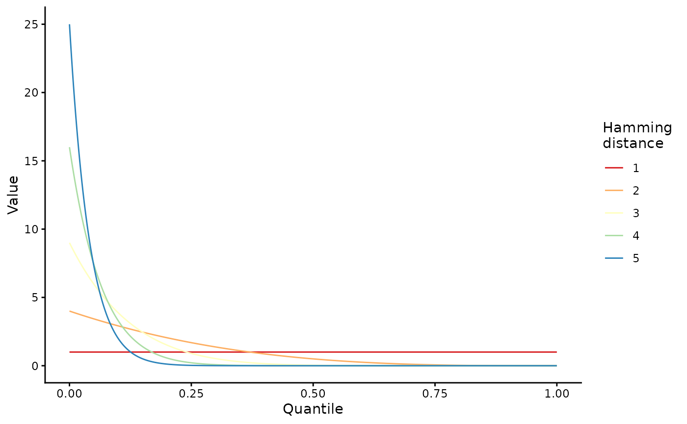

immune_fitness <- run_wavess(
  inf_pop_size = pop,
  samp_scheme = samp,
  founder_seqs = rep(founder_ref$founder, 10),
  b_epitope_locations = epitope_locations
)

The B-cell immune fitness here is now less than 1 after the immune system kicks in:

immune_fitness$counts$mean_b_immune_active
#> [1] 1.0000000 0.7105450 0.7165300 0.7066007

Please note that the model is very sensitive to the maximum antibody immune fitness cost for a given epitope.

T-cell immune fitness

If you specify t_epitope_locations, T-cell immunity will also be modeled and the output will additionally include T-cell immune fitness summaries in the mean_t_immune_active column of the counts tibble and the t_immune column of the fitness tibble.

When modeling the CTL response, we recommend making the conserved cost and the maximum T-cell immune cost the same as it is unclear that one selective pressure always dominates over the other. Below we use 0.5 for both.

Here is a minimal example using a toy T-cell epitope tibble (matching the structure built in vignette("prepare_input_data")):

t_epitope_locations <- data.frame(
  start = c(303, 303, 345, 345, 828, 828),
  days_to_full_potency = c(4, 4, 11, 11, 4, 4),
  escape_position = c(2, 9, 2, 9, 2, 9),
  recognized_aa = c("M", "L", "P", "L", "A", "L")
)

tcell_fitness <- run_wavess(
  inf_pop_size = pop,
  samp_scheme = samp %>% mutate(day = c(0, 1, 2, 3)),
  founder_seqs = rep(founder_ref$founder, 10),
  t_epitope_locations = t_epitope_locations,
  t_max_immune_cost = 0.5,
  conserved_cost = 0.5
)

tcell_fitness$counts$mean_t_immune_active
#> [1] 1.0000000 0.7308239 0.5113636 0.3373580

Multiple selective pressures at once

You can also include multiple selective pressures at once by using multiple of the arguments described above.

Events defined by rates

There are several events that can occur during within-host evolution that are defined by rates of occurrence (which are converted into per-generation probabilities). These include the mutation rate (mut_rate), the recombination rate (recomb_rate), and various rates related to latent cell dynamics (act_to_lat, lat_to_act, lat_prolif, lat_die). Each of these can be turned off by setting the respective rate value to 0. The simulation starts with 0 latent cells, so setting act_to_lat will turn latent cell dynamics off.

Variable recombination rate

The recombination rate modeled by wavess is an effective recombination rate - one number that takes into account the rate of co-infection followed by recombination. By default, the recombination rate is the same across the entire sequence. This occurs whenever the input value is a single number. If you’d like to vary the recombination rate across the sequence, you can input a vector of rates where each element in the vector is a breakpoint-specific recombination rate. In this case, the length of the vector should be one fewer than the number of basepairs in the founder sequence. Here’s an example:

variable_recomb <- run_wavess(
  inf_pop_size = pop,
  samp_scheme = samp,
  founder_seqs = rep(founder_ref$founder, 10),
  recomb_rate = c(rep(1.5e-5, 1000), 1e-4, rep(1.5e-5, 501))
)

Note that inputting a vector for recomb_rate also allows you to simulate reassortment of a segmented virus. In this case, the “recombination rate” between two segments is the rate of co-infection followed by rassortment, and the rate within a segment is the rate of co-infection followed by recombination within that segment.

Alternatively, if you want to model two genes separated by n bases that are not modeled (i.e. not included in the founder sequence), then the recombination rate between the two genes is base_rate*(n+1). Here is example code that preps an input founder sequence where pol and gp120 are spliced together with a higher recombination rate between the genes.

Seed

A seed can be set for reproducibility using the seed argument.

Next: analyzing the outputs

Next, check out vignette("analyze_output") for various ways to visualize and analyze the output data.